INTRODUCTION TO ECONOMY

The Origin and Meaning of Economics

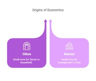
The word ‘Economics’ originates from the Greek word ‘Oikonomikos’, which is a combination of:

• • Oikos: meaning ‘home’
  • Nomos: meaning ‘management’. Thus, the term translates to ‘home management.’

Definition of Economics

      Economics is the study of how individuals and societies make choices, with or without the use of money, to allocate scarce productive resources that have alternative uses. These resources are employed to:

1. Produce various commodities over time, and

2. Distribute them for consumption—either now or in the future—among different persons or groups in society.

Core Focus of Economics

• • Economics involves analyzing the costs and benefits associated with improving patterns of resource allocation.
  • It addresses questions related to scarcity, resource utilization, and decision-making in the face of competing alternatives.

Types of Economics

1. Microeconomics

Etymology:

• • Derived from the Greek word “micro,” meaning “small.”

Definition:

• • Microeconomics focuses on how supply and demand interact within individual markets and how these interactions determine the price levels of goods and services.

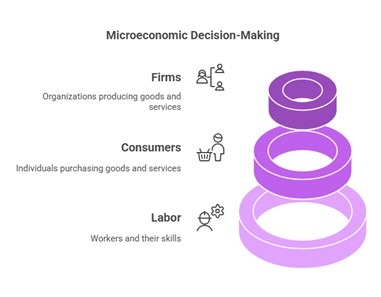
Scope:

It examines the economic behaviour of specific entities, such as:

• • Firms
  • Consumers
  • Labor

Key Focus:

The decision-making processes of individuals and organizations at a smaller, detailed scale.

2. Macroeconomics

Etymology:

• • Derived from the Greek word “makros,” meaning “large.”

Definition:

• • Macroeconomics studies the functioning of the economy as a whole, analyzing broad aggregate indicators and overarching trends.

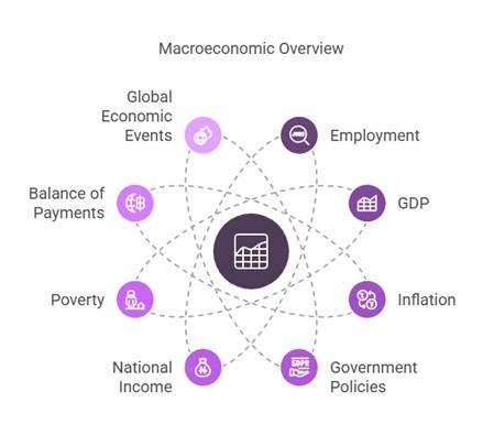
Scope:

It covers topics such as:

• • Employment
  • Gross Domestic Product (GDP)
  • Inflation
  • Government Policies

Key Focus:

• • National income and economic performance
  • Issues like poverty and the balance of payments
  • The impact of global economic events on the national economy.

Key Differences between Microeconomics and Macroeconomics

Other Branches of Economics

     Different economic systems have evolved based on the dominant views and production patterns of various countries. These systems help organize economies in unique ways.

1. Capitalist Economy (Market Economy)

Origin:

• • Associated with the famous work “Wealth of Nations” (1776) by Scottish philosopher and economist Adam Smith.

Definition:

• • An economic system where goods and services are produced and distributed through private or corporate ownership.

Key Features:

• • Free enterprise: Minimal government interference; the economy operates based on supply and demand to meet people’s needs.
  • Market competition: Drives innovation and efficiency for public welfare.

Example:

• • The United States adopted this principle after gaining independence.

2. Socialist Economy (State Economy)

Origin:

• • Proposed by German philosopher Karl Marx.

Definition:

• • An economic system where the means of production are socially owned and operated to fulfill human needs rather than generate profits.
  • Involves collective ownership of resources, with a significant role of the state in managing the economy.

Key Features:

• • Advocates class struggle and revolution to establish a cooperative society.
  • Promotes centralized planning and cooperation over competition.

Examples:

• • Communism was prevalent in the former USSR and currently exists in China and Cuba.

Alternate Names:

• • Centralized economy, Non-market economy.

3. Mixed Economy

Definition:

• • A hybrid system combining features of both public (government-controlled) and private (individually managed) sectors.

Origin:

• • Inspired by John Maynard Keynes, who proposed modifications to address the limitations of pure capitalism.

Key Features:

• • Dual decision-making: Governments manage the public sector while individuals make decisions in the private sector.
  • Balances the government’s role with a market-based economy.

Examples:

• • India and the United Kingdom operate as mixed economies.
  • In India, the economy incorporates Gandhian socialism, emphasizing justice and equality.
  • Since independence, India has pursued two primary objectives:
    1. 1. Economic progress: Achieving technological advancement through democratic means.
       2. Social justice: Establishing a social order that offers equal opportunities for all citizens.

Sectors of the Economy

       Economic activities are categorized into various sectors to highlight the proportion of the population engaged in specific activities. The Indian economy is divided into five major sectors: the Primary, Secondary, Tertiary, Quaternary, and Quinary sectors.

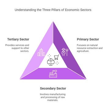
1. PRIMARY SECTOR

• • Involves the extraction or harvesting of natural resources from the Earth.
  • Focuses on the production of raw materials.

Examples of activities:

• • Agriculture, mining, forestry, fishing, etc.

2. SECONDARY SECTOR

• • Involves the production of finished goods through manufacturing, processing, and construction activities.

Examples of activities:

• • Metalworking, automobile production, textiles, shipbuilding, etc.

3. TERTIARY SECTOR

• • Commonly referred to as the service sector.
  • Involves providing services to individuals and businesses.

Examples of activities:

• • Retail, transportation, entertainment, banking, tourism, etc.
  • In advanced economies, the tertiary sector is the largest in terms of production and employment.

4. QUATERNARY SECTOR

• • Comprises intellectual and knowledge-based activities.

Examples of activities:

• • Research and development, consulting, financial planning, education, etc.

5. QUINARY SECTOR

• • Represents the highest levels of decision-making in a country.
  • Includes key roles in government, media, and top academic institutions.

Examples of activities:

• • Policy formulation, leadership roles in government, high-level university officials, etc.

Basic Concepts of Economics

1. Goods

Definition:

• • Goods are physical, tangible products produced and consumed in an economy.

Types of Goods:

1. Consumer Goods:

1. • Purchased by individuals or households for personal consumption.
   • Directly satisfy human needs and desires.
   • Examples: Food items, clothing, electronics (like smartphones and televisions), furniture, and household appliances.

2. Capital Goods:

1. • Used by businesses to produce other goods or provide services.
   • Not for direct consumption but essential in the production process.
   • Examples: Machinery, tools, buildings, equipment (e.g., a farmer’s tractor, a printing press for publishing).

Classification Based on Durability:

1. Durable Goods:

1. • Long-lasting goods with a lifespan of more than three years.
   • Examples: Cars, refrigerators, furniture, laptops.

2. Non-Durable Goods:

1. • Goods with a short lifespan or consumed quickly.
   • Examples: Food, beverages, toiletries, stationery.

Classification Based on Rivalry and Excludability:

1. Private Goods:

1. • Rivalrous and excludable.
   • Ownership is limited to those who purchase them, and consumption by one person reduces availability for others.
   • Examples: Clothing, personal electronics, privately owned vehicles.

2. Public Goods:

1. • Non-rivalrous and non-excludable.
   • Provided by the government or public institutions for the benefit of all.
   • One person’s use does not reduce availability for others.
   • Examples: Street lighting, national defense, public parks.

3. Common Goods:

1. • Rivalrous but non-excludable.
   • Available for everyone to use, but consumption by one reduces availability for others.
   • Often face overuse or depletion issues.
   • Examples: Fisheries, forests, grazing lands.

4. Club Goods:

1. • Excludable but non-rivalrous.
   • Provided by private organizations or clubs. Access is restricted to members or subscribers.
   • Examples: Cable TV, subscription services (like Netflix), private golf courses.

2. Services

Definition:

• • Services are intangible activities performed by individuals or businesses to fulfill needs or wants.

Key Characteristics:

1. Intangible Nature: Services cannot be seen, touched, or stored.

2. Real-Time Production & Consumption: Services are often produced and consumed simultaneously (e.g., a haircut or a live performance).

3. Human Interaction: Relies heavily on human skills, expertise, and interactions.

4. Examples: Hair salons, education, banking, healthcare, transportation, entertainment.

3. Utility

Definition:

• • Utility refers to the satisfaction or usefulness a person derives from consuming a good or service.

Key Concepts:

1. Marginal Utility:

1. • The additional satisfaction gained from consuming one more unit of a good or service.
   • Helps understand how satisfaction changes with increased consumption.

2. Law of Diminishing Marginal Utility:

1. • As more units of a good or service are consumed, the additional satisfaction (marginal utility) derived from each unit decreases.
   • Explains why people tend to seek variety and why demand decreases as consumption increases.

Example (Pizza):

• • First Slice: High satisfaction, assigned 10 utility units.
  • Second Slice: Slightly less satisfaction, assigned 8 utility units.
  • Third Slice: Even less satisfaction, assigned 5 utility units.

Implications:

• • Explains consumer behavior and decision-making.
  • Encourages exploration of alternative goods/services to maintain satisfaction levels.

4. Cost

Definition:

• • Cost refers to the expenses incurred in producing goods or services.

Types of Costs:

1. Fixed Costs:

1. • Do not vary with the level of production.
   • Examples: Rent, salaries, equipment leases.

2. Variable Costs:

1. • Vary directly with the level of production.
   • Examples: Raw materials, utility bills, wages based on production levels.

3. Total Costs:

1. • Sum of fixed and variable costs.

4. Average Cost:

1. • Calculated by dividing total cost by the quantity of goods produced.
   • Provides insight into the cost per unit of production.

Opportunity Cost:

• • Represents the value of the next best alternative forgone when making a decision.
  • Highlights the benefits or profits that could have been gained by choosing another option.
  • Example: If you start a bakery, your opportunity cost might be the income you could have earned as a chef in a restaurant.

5. Price

Definition:

• • Price is the monetary value assigned to a good or service, representing the exchange rate agreed upon by buyers and sellers.

Factors Influencing Price:

1. Supply and Demand:

1. • High demand and low supply = Higher prices.
   • Low demand and high supply = Lower prices.

2. Production Costs:

1. • Higher production costs typically lead to higher prices.

3. Competition:

1. • Intense competition can drive prices lower, while monopolies may set higher prices.

4. Government Intervention:

1. • Taxes, subsidies, or price ceilings/floors can influence market prices.

5. Market Conditions:

1. • Economic factors like inflation, exchange rates, or consumer trends can impact prices.

Concepts of Microeconomics

1. Demand

Definition:
    The Law of Demand is indeed a fundamental concept in economics. It highlights the inverse relationship between the price of a good or service and the quantity demanded by consumers. This principle assumes that all other factors affecting demand are constant (ceteris paribus). For instance, when the price of smartphones decreases, consumers are more inclined to buy more because they perceive greater value or affordability, thus increasing the quantity demanded.

   Conversely, if smartphone prices rise, consumers might seek alternatives or forego purchases, thereby decreasing the quantity demanded. This relationship is visualized as a downward-sloping demand curve on a graph where price is on the vertical axis and quantity demanded is on the horizontal axis. Exceptions to this principle can occur due to factors such as changes in consumer preferences, income levels, or the presence of substitute goods.

Determinants of Demand:

1. Price of the Product:

1. • The primary factor influencing demand.
   • When the price decreases, the quantity demanded typically increases, and vice versa.
   • Example: A drop in smartphone prices may lead to higher sales.

2. Income:

1. • Consumer income affects purchasing power.
   • Higher income generally increases demand for goods, especially luxury items.
   • Example: As salaries rise, people may buy more expensive jewelry or premium gadgets.

3. Price of Related Goods:

1. • Substitutes: Goods that can replace each other (e.g., tea and coffee). An increase in the price of one leads to higher demand for the other.
   • Complements: Goods that are used together (e.g., smartphones and mobile data plans). A decrease in the price of one can boost demand for the other.

4. Consumer Preferences and Tastes:

1. • Preferences influenced by trends, advertising, and societal norms can impact demand.
   • Example: A new fashion trend increases demand for specific clothing styles.

5. Population:

1. • The size and demographics of a population affect overall demand.
   • Example: A new housing development increases demand for furniture and appliances.

2. Elasticity of Demand

Definition:
     Elasticity in economics measures how the quantity demanded or supplied responds to changes in price. It provides insight into consumer and producer behaviour, particularly in relation to pricing strategies and tax models.

Types of Elasticity of Demand:

1. Elastic Demand:

1. • A small price change causes a significant change in quantity demanded.
   • Consumers are highly sensitive to price changes.
   • Example: If luxury car prices rise, consumers may switch to cheaper alternatives or delay purchases.

2. Inelastic Demand:

1. • A price change causes a relatively small change in quantity demanded.
   • Applies to necessities that people continue to purchase despite price increases.
   • Example: Basic groceries like rice and bread.

3. Unit Elastic Demand:

1. • A price change results in a proportional change in quantity demanded.
   • Example: A 10% price increase leads to a 10% decrease in quantity demanded.

Demand curve

      The demand curve generally reflects an inverse relationship between price and quantity demanded, typically sloping downward from left to right. This implies that when the price of a product decreases, the quantity demanded usually increases, and conversely, when the price increases, the quantity demanded tends to decrease.

    However, certain scenarios lead to “exceptional demand curves,” where the curve slopes upward from left to right. In these situations, a decrease in price could result in lower demand, and an increase in price might lead to higher demand.

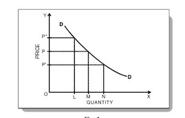
Key Features:

• • Downward-Sloping Curve (D): This indicates the inverse relationship between price and quantity demanded—meaning as price decreases, quantity demanded increases.
  • Axes:
    • • • Y-Axis (Price): Represents the price of the good or service.
        • X-Axis (Quantity): Represents the quantity demanded.
  • Points (L, M, N): These points could represent specific quantities demanded at different price levels marked as P, P’, etc.

3. Exceptions to the Law of Demand

Although the law of demand generally holds true, some exceptions exist:

1. Giffen Goods:

1. • These are inferior goods that defy the law of demand.
   • When the price rises, the quantity demanded also increases because these goods are essential staples for low-income consumers.
   • Example: An increase in rice prices might force low-income families to buy more rice and less of other expensive foods.

2. Veblen Goods:

1. • Luxury goods that are more desirable as their prices increase.
   • High prices serve as a status symbol, attracting consumers seeking prestige.
   • Example: Designer handbags or luxury watches become more appealing as prices rise.

The speculative effect can alter the shape of the demand curve based on consumers’ expectations regarding future events. When the price of a commodity is rising, consumers might choose to purchase more of it, anticipating that prices will continue to climb. This behavior leads to an upward-sloping demand curve.

A relevant example is the real estate market. When housing prices begin to rise, potential homebuyers may rush to purchase properties, expecting that prices will keep increasing. This anticipation drives demand higher, illustrating how speculation can reverse the usual demand behavior.

Concepts of Microeconomics

1. Supply

Definition:
    Supply refers to the quantity of a good or service that producers are willing and able to offer for sale at different prices over a specific time period. It reflects the relationship between a product’s price and the quantity producers are ready to produce and sell.

Law of Supply:

• • The law of supply states that there is a direct relationship between the price of a product and the quantity supplied, assuming all other factors remain constant.
  • As the price increases, the quantity supplied increases, and as the price decreases, the quantity supplied decreases.
  • This relationship is represented by the supply curve, which slopes upward.

Determinants of Supply:

1. Price of Inputs:

1. • The cost of resources needed for production.
   • Higher input costs reduce supply, while lower costs increase it.
   • Example: A rise in raw material prices may lead to reduced supply of finished goods.

2. Technology:

1. • Technological advancements improve efficiency, lower costs, and increase supply.
   • Example: Automation in factories can boost production and reduce expenses.

3. Number of Sellers:

1. • More sellers entering the market increases supply; fewer sellers decrease it.
   • Example: The entry of new firms in the solar panel industry increases supply.

4. Expectations:

1. • Future price expectations influence current supply.
   • Example: If producers expect higher future prices, they may reduce current supply to sell later at higher profits.

5. Government Regulations:

1. • Policies such as taxes, subsidies, or restrictions can affect supply.
   • Example: Subsidies for electric vehicles increase their supply, while taxes on tobacco reduce supply.

Elasticity of Supply:

Elasticity of supply measures how responsive the quantity supplied is to changes in price.

1. Elastic Supply:

1. • Quantity supplied is highly responsive to price changes.
   • Example: Farmers planting more crops when prices rise.

2. Inelastic Supply:

1. • Quantity supplied changes only slightly in response to price changes.
   • Example: Limited resources like precious metals show little change in supply even with price increases.

3. Unitary Elastic Supply:

1. • Percentage change in quantity supplied equals the percentage change in price.
   • Example: A 10% price increase leads to a 10% rise in quantity supplied.

Supply curve

     The supply curve illustrates the direct relationship between price and quantity supplied. As prices increase, suppliers are willing to offer more of a good or service.

Key Points:

• • Direct Relationship: When the price rises from OP1 to OP2, the quantity supplied increases from OQ1 to OQ2.
  • Upward Sloping: The supply curve typically slopes upwards from left to right, indicating that higher prices incentivize producers to supply more.

This relationship reflects how market dynamics affect supplier behavior, showcasing that as prices go up, supply tends to increase to meet potential demand.

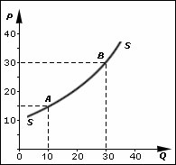
Key Features:

1. Upward-Sloping Curve (S): This indicates a direct relationship between price and quantity supplied, meaning as price increases, the quantity supplied also increases.

2. Axes:

• • Y-Axis (P): Represents the price of the good.
  • X-Axis (Q): Represents the quantity supplied.

3. Points (A, B):

• • Point A: Represents a specific quantity supplied (around 10 units) at a lower price (around 10).
  • Point B: Represents a higher quantity supplied (around 30 units) at a higher price (around 20).

Interpretation:

• • As the price moves from 10 to a higher point (like 20), the quantity supplied increases from a lower amount (like 10) to a higher amount (like 30).
  • This graph visually demonstrates how suppliers respond to price changes, aligning with the law of supply.

2. Market Equilibrium

Definition:
      Market Equilibrium is achieved when the quantity demanded by consumers equals the quantity supplied by producers, determining the market price for a good or service.

Key Features:

1. Equilibrium Point: This is where the demand and supply curves intersect on a graph, indicating the price and quantity where the market is balanced.

Imbalances:

• • Surplus (Excess Supply): Quantity supplied exceeds quantity demanded, leading to downward pressure on prices.
  • Shortage (Excess Demand): Quantity demanded exceeds quantity supplied, causing prices to rise.

Example – Coffee Shop:

• • The coffee shop sets the price of a cup of coffee at $3. At this price, they expect to sell 100 cups per day.
  • If the shop produces 100 cups, all the coffee is sold by the end of the day, indicating a balanced market without leftovers or unmet customer demand.
  • If the price is raised to $4, the shop might produce 80 cups, but customers demand 60 cups, resulting in a surplus.
  • Conversely, if the price drops to $2, the shop could produce 120 cups, but customer demand might only reach 90 cups, leading to a shortage.

Importance:

• • This equilibrium ensures the coffee shop maximizes its profits while meeting customer needs. Price changes can shift this equilibrium point, affecting both supply and demand in the market.

Theory of the Firm

       The Theory of the Firm is a branch of microeconomics that examines the various organizational structures that firms can adopt within different industries. It analyzes how these structures influence decision-making, production efficiency, and overall market behavior.

Key Components:

1. Types of Organizational Structures: This includes sole proprietorships, partnerships, corporations, and cooperatives, each with unique characteristics and implications for management and operations.

2. Decision-Making: The theory looks at how firms make decisions regarding production, pricing, and resource allocation based on their structure and the competitive environment.

3. Efficiency and Competition: It also explores how different structures affect a firm’s efficiency and competitiveness in the market, including factors like economies of scale and market power.

4. Insights into Industry Dynamics: By understanding these organizational forms and their implications, economists can draw conclusions about industry behavior and the effects of regulations and market changes.

This theory provides valuable insights into how firms operate, compete, and adapt within the broader economic landscape.

3. Competition

Definition:
      Competition refers to the rivalry among sellers in the market, aiming to attract buyers and increase sales. It influences prices, quality, and variety.

Types of Market Structures Based on Competition:

1. Perfect Competition:

• • Characteristics:
    • • Many buyers and sellers.
      • Homogeneous (identical) products.
      • No single entity controls prices.
  • Example: Agricultural markets like wheat and rice.

2. Monopolistic Competition:

• • Characteristics:
    • • Many sellers offering similar but differentiated products.
      • Sellers use branding, marketing, and unique features to compete.
  • Example: Fast-food chains like McDonald’s and Burger King.

3. Oligopoly:

• • Characteristics:
    • • A few large sellers dominate the market.
      • Sellers can influence prices and market conditions.
      • The actions of one seller significantly affect others.
  • Example: Automobile industry and smartphone market.

4. Monopoly:

• • Characteristics:
    • • Single seller dominates the entire market.
      • Complete control over price and quantity.
      • Often leads to higher prices and fewer choices for consumers.
  • Example: Public utilities like water or electricity providers in certain regions.

5. Monopsony:

• • Characteristics:
    • • A market with only one buyer and multiple sellers.
      • The buyer has significant control over prices and trade terms.
  • Example: A factory in a small town acting as the sole employer for labor.