PRESSURE
Pressure is a fundamental concept in physics and engineering, defined as the force applied per unit area. It plays a crucial role in fluid mechanics, weather systems, industrial machinery, and even biological processes. The mathematical representation of pressure is:
P=FAP=AF
Where:
- PP = Pressure (Pascals, Pa)
- FF = Force applied (Newtons, N)
- AA = Area over which the force is distributed (square meters, m²)
Units of Pressure
- Pascal (Pa) – The SI unit, where 1 Pa = 1 N/m².
- Atmosphere (atm) – Standard atmospheric pressure at sea level is 1 atm = 1.013 × 10⁵ Pa.
- Bar (bar) – Commonly used in meteorology, 1 bar ≈ 1 atm.
- mmHg (millimeters of mercury) – Used in medicine (blood pressure) and weather reports.
Fluid Flow and Pressure Differences
Fluids (liquids and gases) naturally move from high-pressure regions to low-pressure regions. This principle governs numerous natural and man-made systems:
Examples of Fluid Flow Due to Pressure Differences
- Blood Circulation – The heart pumps blood from high-pressure arteries to low-pressure veins.
- Water Supply Systems – Water flows from reservoirs (high pressure) through pipes to homes (low pressure).
- Respiratory System – Air moves into the lungs when diaphragm contraction lowers internal pressure.
Altitude and Atmospheric Pressure
How Pressure Changes with Altitude
- As altitude increases, air density decreases, leading to lower atmospheric pressure.
- At Mount Everest’s summit (8,848 m), pressure is only about 30% of sea-level pressure.
Effects on Humans:
- Reduced oxygen availability causes altitude sickness.
- Boiling point of water decreases, affecting cooking (discussed below).
Boiling Point Variation with Pressure
- Lower Pressure = Lower Boiling Point
- At high altitudes, water boils below 100°C, making cooking slower (e.g., rice takes longer).
- Higher Pressure = Higher Boiling Point
- Pressure cookers increase internal pressure, raising the boiling point above 100°C, thus cooking food faster.
- Lower Pressure = Lower Boiling Point
Applications of Pressure in Daily Life
1. Hydraulic Lifts (Pascal’s Principle)
- How It Works: A small force applied to a small piston generates a larger force on a bigger piston due to fluid pressure.
- Applications:
- Car lifts in auto repair shops.
- Elevators and heavy machinery.
2. Drinking Through a Straw
- Sucking creates a low-pressure zone inside the straw.
- Atmospheric pressure pushes the liquid up into your mouth.
3. Pressure Cookers
- Principle: Sealed container increases pressure, raising the boiling point of water.
- Benefits:
- Faster cooking (rice, lentils, meat).
- Energy-efficient (less fuel required).
4.Weather Systems: Land and Sea Breezes
- Sea Breeze (Daytime):
- Land heats faster → Low pressure over land.
- Cooler sea air (high pressure) moves inland.
- Land Breeze (Nighttime):
- Land cools faster → High pressure over land.
- Warmer sea air (low pressure) moves toward the sea.
- Sea Breeze (Daytime):
Cloud Formation, Rainfall, and Desert Climates
How Clouds Form
1. Warm, moist air rises (low-pressure zone).
2. Air expands and cools at higher altitudes.
3. Water vapor condenses into tiny droplets → Clouds form.
4. Droplets combine → Become heavy → Rainfall.
Why Deserts Exist
- High-pressure zones cause dry, descending air.
- Low humidity prevents cloud formation.
- Result: Minimal rainfall (e.g., Sahara, Atacama deserts).
Key Takeaways
Concept | Explanation | Real-World Example |
Pressure Definition | Force per unit area (P=F/AP=F/A) | Hydraulic lifts |
Altitude & Pressure | Pressure decreases with height | Longer rice cooking at high altitudes |
Boiling Point & Pressure | Higher pressure = higher boiling point | Pressure cookers |
Fluid Flow | Moves from high to low pressure | Blood circulation |
Weather Systems | Land/sea breezes due to pressure differences | Coastal wind patterns |
Cloud Formation | Low pressure → Rising air → Condensation | Rain and thunderstorms |
Desert Formation | High pressure → Dry descending air | Sahara Desert |
Pressure is a versatile and essential concept influencing everything from cooking to weather patterns. Understanding how it works helps explain:
- Why planes need pressurized cabins at high altitudes.
- How hydraulic machines lift heavy loads with minimal effort.
- Why deserts are dry while rainforests receive heavy rainfall.

FLUID DYNAMICS
Laminar Flow:
Laminar flow, also known as streamline flow, describes the smooth, orderly movement of a fluid in parallel layers with no disruption between them. Unlike turbulent flow (chaotic and mixed), laminar flow maintains steady velocity and predictable motion, making it essential in engineering, medicine, and aerodynamics.
Key Characteristics of Laminar Flow
1. Layered Motion
- Fluid moves in parallel layers (laminae) without mixing.
- Example: Honey pouring slowly from a jar.
2. Constant Velocity
- Each particle follows a smooth, unchanging path (streamline).
3. Low Reynolds Number (Re < 2,000)
- The Reynolds number (ReRe) determines flow type:
Re=ρvLμRe=μρvL
- ρρ = Fluid density
- vv = Flow velocity
- LL = Characteristic length (e.g., pipe diameter)
- μμ = Dynamic viscosity
4. No Eddies or Swirls
- Minimal energy loss due to friction.
Examples of Laminar Flow in Nature and Technology
1. Blood Flow in Capillaries
Why Laminar?
- Narrow vessels + low velocity → Low Reynolds number.
- Ensures efficient oxygen delivery without damaging cells.
2. Airflow Over Airplane Wings (At Low Speeds)
- Laminar Flow Wings reduce drag, improving fuel efficiency.
3. Water Flow in Pipes (Low Velocity)
- Household plumbing often exhibits laminar flow.
4. Industrial Processes
- Chemical Manufacturing – Precise fluid control in reactors.
- Microfluidics – Used in lab-on-a-chip devices.
Why Does Laminar Flow Matter?
1. Medical Applications
- IV Drips: Laminar flow ensures controlled drug delivery.
- Ventilators: Prevents air turbulence in patient airways.
2. Engineering & Design
- Aerodynamics: Laminar wings reduce drag in aircraft.
- Hydraulic Systems: Minimizes energy loss in pipes.
3. Environmental Science
- River Ecosystems: Slow, laminar flows support certain aquatic life.
How to Identify Laminar Flow
1. Dye Test
- Inject dye into fluid → If it moves in a straight line, flow is laminar.
2. Reynolds Number Calculation
- Compute ReRe: Values below 2,000 indicate laminar flow.
Laminar flow’s predictable, energy-efficient nature makes it invaluable in fields ranging from medicine to aerospace. Understanding its principles helps optimize:
- Medical devices (e.g., stents, ventilators).
- Transport systems (e.g., planes, pipelines).
- Industrial processes (e.g., chemical mixing).
By controlling factors like viscosity, velocity, and pipe diameter, engineers and scientists harness laminar flow for safer, more efficient systems.

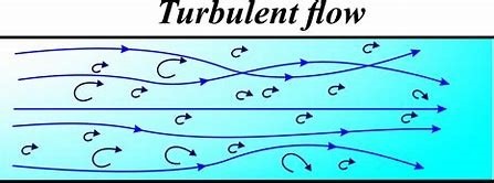
Turbulent Flow:
Turbulent flow represents one of the most complex and fascinating phenomena in fluid dynamics. Unlike its orderly counterpart (laminar flow), turbulent flow is characterized by chaotic motion, irregular velocity fluctuations, and swirling eddies. This type of flow occurs when inertial forces dominate viscous forces, typically at high Reynolds numbers (Re > 4,000).
Turbulence plays a crucial role in nature and technology – from weather systems to industrial processes. Understanding its behavior helps engineers design more efficient systems while explaining many natural phenomena.
Key Characteristics of Turbulent Flow
1. Chaotic Motion
- Fluid particles follow unpredictable, erratic paths
- No discernible pattern or streamline consistency
2. Velocity Fluctuations
- Rapid, random changes in speed and direction at any point
- Creates instantaneous variations in flow properties
3. Eddy Formation
- Swirling vortices of different sizes form and dissipate
- Energy cascades from large to small eddies (Kolmogorov’s theory)
4. High Mixing Capacity
- Excellent for mass and heat transfer applications
- Causes rapid dispersion of pollutants in atmosphere/water
5. Energy Dissipation
- Significant energy loss due to internal friction
- Requires more power to maintain flow compared to laminar.
The Science Behind Turbulence: Reynolds Number
The transition from laminar to turbulent flow is predicted by the Reynolds number:
Re=ρvLμRe=μρvL
Where:
- ρ = fluid density (kg/m³)
- v = flow velocity (m/s)
- L = characteristic length (e.g., pipe diameter)
- μ = dynamic viscosity (Pa·s)
Flow Regimes:
- Re < 2,000: Laminar flow
- 2,000 < Re < 4,000: Transitional flow
- Re > 4,000: Turbulent flow
Real-World Examples of Turbulent Flow
1. Natural Phenomena
River Currents:
- Fast-moving water around rocks/bends creates whirlpools
- Essential for nutrient mixing in ecosystems
Atmospheric Turbulence:
- Causes bumpy airplane rides
- Influences weather patterns and storm development
Ocean Waves:
- Breaking waves demonstrate turbulent energy dissipation
2. Engineering Applications
Pipe Flow Systems:
- Water distribution networks experience turbulence at high velocities
- Increases pumping costs but improves mixing.
Aerodynamics:
- Airflow over vehicles/aircraft at high speeds
- Boundary layer turbulence affects drag and fuel efficiency.
Industrial Mixers:
- Turbulence ensures thorough blending of liquids/gases.
3. Biological Systems
Human Airways:
- Breathing at high rates (exercise) causes turbulent flow
- Enhances oxygen-carbon dioxide exchange
Blood Flow:
- Occurs in large arteries during peak cardiac output
- Pathological turbulence may indicate heart valve disorders.
The Importance of Studying Turbulence
1. Energy Efficiency
- Understanding turbulence helps reduce energy losses in pipelines
- Improves designs of aircraft and vehicles
2. Environmental Protection
- Predicts pollutant dispersion in air/water
- Helps design effective wastewater treatment
3. Medical Advances
- Analysis of blood flow turbulence aids cardiovascular diagnosis
- Improves ventilator designs for critical care
4. Industrial Optimization
- Enhances chemical mixing processes
- Refines combustion systems in engines.
Challenges in Turbulence Research
Despite over a century of study, turbulence remains one of classical physics’ unsolved problems because:
- Extremely complex mathematical modeling
- Sensitive dependence on initial conditions
- Wide range of interacting scales (from large eddies to tiny vortices)
- Difficult to simulate accurately even with supercomputers.
Modern approaches include:
- Computational Fluid Dynamics (CFD)
- Particle Image Velocimetry (PIV)
- Machine learning applications
While turbulent flow presents challenges, its high mixing capability makes it invaluable across industries. From ensuring efficient fuel combustion to explaining weather patterns, understanding turbulence helps us:
- Design better transportation systems
- Improve environmental management
- Advance medical technologies
- Optimize industrial processes
Diffusion
Diffusion is one of nature’s most essential transport mechanisms, governing processes from cellular respiration to industrial chemical engineering. This spontaneous process involves the net movement of particles (atoms, molecules, or ions) from regions of high concentration to low concentration due to random thermal motion, ultimately achieving equilibrium.
The Science Behind Diffusion
1. Molecular Basis of Diffusion
- Thermal Energy Driven: Particles constantly move due to kinetic energy (faster at higher temperatures)
- Random Walk Motion: Particles follow unpredictable paths from collisions
- Net Movement: While individual particle motion is random, the population moves down concentration gradients
2. Fick’s Laws of Diffusion
The mathematical foundation of diffusion was established by Adolf Fick in 1855:
First Law (Steady-State Diffusion):
J=−DdCdxJ=−DdxdC
Where:
- JJ = Diffusion flux (amount of substance per unit area per time)
- DD = Diffusion coefficient (depends on material and temperature)
- dCdxdxdC = Concentration gradient
Second Law (Non-Steady-State Diffusion):
- ∂C∂t=D∂2C∂x2∂t∂C=D∂x2∂2C
- Describes how concentration changes over time
Types of Diffusion
Type | Description | Example |
Simple Diffusion | Direct movement through medium | Perfume spreading in air |
Facilitated Diffusion | Uses membrane transport proteins | Glucose entering cells |
Osmosis | Water diffusion through membranes | Plant root water absorption |
Electrodiffusion | Ions moving under concentration & electrical gradients | Nerve impulse transmission |
Factors Affecting Diffusion Rates
1. Concentration Gradient
- Steeper gradient → Faster diffusion
(Example: Strong coffee aroma spreads faster than weak)
- Steeper gradient → Faster diffusion
2. Temperature
- Higher temperature → Increased kinetic energy → Faster diffusion
(Food coloring mixes faster in hot vs. cold water)
- Higher temperature → Increased kinetic energy → Faster diffusion
3. Medium Properties
- Gas > Liquid > Solid diffusion rates
- Viscosity inversely affects speed
4. Particle Characteristics
- Smaller/lighter particles diffuse faster (Graham’s Law)
- Nonpolar molecules diffuse through membranes more easily.
5. Diffusion Distance
- Shorter paths → Faster equilibration
(Evolution designed alveoli as thin sacs for rapid gas exchange)
- Shorter paths → Faster equilibration
Biological Importance of Diffusion
1. Respiratory System
Alveolar Gas Exchange:
- Oxygen diffuses from air (high pO₂) to blood (low pO₂)
- CO₂ diffuses in opposite direction
- Membrane thickness < 0.5μm for efficiency.
2. Cellular Nutrition
- Nutrient uptake (e.g., intestinal villi absorbing glucose)
- Waste removal (e.g., urea exiting cells)
3. Nervous System
- Neurotransmitter diffusion across synapses
- Maintenance of ion gradients for action potentials
4. Plant Physiology
- Stomatal CO₂ uptake for photosynthesis
- Root nutrient absorption from soil
Industrial & Technological Applications
1. Chemical Engineering
- Separation processes (e.g., dialysis, distillation)
- Catalyst design for optimal molecular access.
2. Materials Science
- Semiconductor doping
- Metal alloy hardening via carbon diffusion
3. Medical Technologies
- Drug delivery systems (transdermal patches)
- Hemodialysis machines
4. Environmental Engineering
- Air pollution dispersion modeling
- Groundwater contaminant transport
Mathematical Modeling of Diffusion
Advanced applications use:
- Monte Carlo simulations for particle trajectories
- Finite element analysis for complex geometries
- Fractal mathematics for porous media diffusion.
The Universal Role of Diffusion
From subcellular processes to galactic gas clouds, diffusion represents a fundamental mechanism of nature. Its principles enable:
- Life-sustaining biological processes
- Efficient industrial operations
- Advanced material designs
- Environmental protection strategies
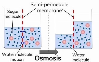
Osmosis:
Osmosis represents one of nature’s most elegant transport mechanisms – the selective movement of water molecules across semipermeable membranes to equalize solute concentrations. This passive process powers essential biological functions from plant hydration to human kidney operations, while also finding applications in industrial purification systems.
The Science of Osmosis Explained
1. Fundamental Principles
- Semipermeable Membranes: Allow water but block most solutes
- Water Potential Gradient: Drives water from high Ψ (low solute) to low Ψ (high solute)
- Dynamic Equilibrium: Net water movement ceases when concentrations balance.
2. The Osmotic Pressure Equation
Van’t Hoff’s law quantifies osmotic pressure (π):
π=iCRTπ=iCRT
Where:
- i = van’t Hoff factor (ions per molecule)
- C = molar concentration (mol/L)
- R = gas constant (0.0821 L·atm/K·mol)
- T = temperature (Kelvin)
Types of Osmotic Environments
Solution Type | Water Movement | Cell Response | Example |
Hypotonic | Into cell | Swelling/lysis | Distilled water exposure |
Isotonic | Balanced flow | Normal shape | Physiological saline (0.9% NaCl) |
Hypertonic | Out of cell | Shrinkage (crenation) | Seawater immersion |
Biological Significance of Osmosis
1. Plant Physiology
Root Water Uptake:
- Root hair cells maintain higher solute concentration
- Creates continuous water inflow (root pressure up to 0.2 MPa)
- Enables capillary action in xylem vessels
Turgor Pressure:
- Central vacuole expansion creates structural rigidity
- Wilting occurs when Ψcell > Ψenvironment
2. Human Physiology
Kidney Function:
- Descending loop of Henle: Water exits via osmosis
- Collecting duct: ADH-regulated water reabsorption
Red Blood Cells:
- 0.9% NaCl maintains isotonic conditions
- Hemolysis occurs in hypotonic solutions
3. Microbial Survival
- Halophiles maintain high intracellular KCl
- Contractile vacuoles in freshwater protists
Industrial and Medical Applications
1. Water Purification
Reverse Osmosis (RO):
- Applies external pressure > π to desalinate water
- Removes 95-99% of dissolved salts
- Global capacity exceeds 100 million m³/day
2. Medical Therapeutics
Intravenous Fluids:
- Lactated Ringer’s (273 mOsm/L) for blood volume expansion
- Hypertonic saline (3-23.4%) for cerebral edema
Dialysis:
- Countercurrent osmotic exchange removes uremic toxins
3. Food Preservation
- Sugar/salt curing creates hypertonic environments
- Inhibits microbial growth via plasmolysis
Osmosis in Nature
1. Mangrove Adaptation
- Salt-excreting leaves maintain Ψleaf < Ψseawater
- Prop roots develop ultrafiltration membranes
2. Desert Plant Strategies
- Thick cuticles reduce transpirational water loss
- CAM photosynthesis minimizes stomatal opening
3. Marine Organisms
- Shark rectal gland excretes concentrated NaCl
- Seabirds drink seawater using salt glands
Experimental Demonstrations
1. Classic Egg Membrane Lab
- Decalcify eggs in vinegar (semipermeable membrane)
- Measure mass changes in corn syrup vs. distilled water
- Calculate osmotic potential differences
2. Potato Osmolarity Test
- Determine isotonic point via mass change series
- Plot water potential vs. sucrose concentration
Mathematical Modeling
1. Kedem-Katchalsky Equations
Describe coupled solute-solvent transport:
Jv=Lp(Δπ−σΔP)Jv=Lp(Δπ−σΔP)Js=ωΔC+(1−σ)CJvJs=ωΔC+(1−σ)CJv
Where:
- J<sub>v</sub> = volume flux
- L<sub>p</sub> = hydraulic conductivity
- σ = reflection coefficient
2. Computational Approaches
- Finite element analysis of membrane systems
- Molecular dynamics simulations of aquaporins
Current Research Frontiers
1. Biomimetic Membranes:
- Aquaporin-incorporated filters for energy-efficient desalination
2. Osmotic Power Generation:
- Pressure-retarded osmosis (PRO) at river estuaries
- Potential 1,600 TWh/year global capacity
3. Drug Delivery Systems:
- Osmotic pumps for controlled release (e.g., OROS® technology)
Comparison with Related Processes
Process | Driving Force | Membrane Requirement | Example |
Osmosis | Water potential gradient | Semipermeable | Plant water uptake |
Dialysis | Concentration gradient | Selective permeable | Kidney filtration |
Ultrafiltration | Pressure gradient | Microporous | Water treatment |
From sustaining cellular life to enabling cutting-edge technologies, osmosis remains a cornerstone process across disciplines. Its principles continue to inspire solutions for:
- Global water scarcity (advanced RO systems)
- Sustainable energy (blue energy harvesting)
- Precision medicine (smart drug delivery)
Surface Tension
Surface tension is one of the most fascinating and observable fluid properties, governing phenomena from morning dewdrops to industrial processes. This macroscopic manifestation of molecular forces creates a liquid’s “elastic skin,” enabling remarkable behaviors that defy everyday expectations about liquids.
The Molecular Origin of Surface Tension
1. Cohesive Forces at Work
- Interior Molecules: Experience balanced attractive forces from all directions
- Surface Molecules: Face net inward pull due to missing upward attractions
- Energy Minimization: System naturally reduces surface area (spontaneous process)
2. Quantitative Definition
Surface tension (γ) is measured as:
γ=FLγ=LF
Where:
- F = Force parallel to surface
- L = Length along which force acts
Units: N/m (SI) or dyn/cm (CGS)
3. Thermodynamic Perspective
γ=(∂G∂A)T,P,nγ=(∂A∂G)T,P,n
- G = Gibbs free energy
- A = Surface area
- Represents work needed to expand surface
Remarkable Manifestations of Surface Tension
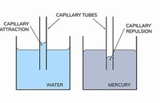
1. Capillary Action
- Concave Meniscus: Water climbs glass tubes (adhesion > cohesion)
- Convex Meniscus: Mercury depresses in glass (cohesion > adhesion)
- Jurín’s Law: Height of rise h=2γcosθρgrh=ρgr2γcosθ
2. Biological Adaptations
- Water Striders: Microsetae create superhydrophobic legs (contact angle ~167°)
- Lung Surfactants: DPPC reduces alveolar surface tension to ~25 mN/m
- Plant Xylem: Negative pressure from transpiration pulls water upward
3. Industrial Applications
- Inkjet Printing: Precise droplet formation (Weber number control)
- Froth Flotation: Mineral separation via bubble adhesion
- Electroplating: Surface tension affects coating uniformity
Surface Tension Values (20°C)
Liquid | Surface Tension (mN/m) | Notable Property |
Water | 72.8 | Hydrogen bonding network |
Mercury | 485 | Exceptionally high metallic bonding |
Ethanol | 22.1 | Significant hydrogen bonding |
Liquid Helium | 0.12 | Weak van der Waals forces |
Liquid Steel | ~1,500 | Extreme metallic bonding |
The Physics of Droplet Formation
1. Spherical Minimization
- Laplace Pressure: ΔP=2γrΔP=r2γ
- Explains why smaller droplets have higher internal pressure
- Rayleigh-Plateau Instability: Explains liquid jet breakup into droplets
- Laplace Pressure: ΔP=2γrΔP=r2γ
2. Contact Angle Phenomena
- Young’s Equation: γsv=γsl+γlvcosθγsv=γsl+γlvcosθ
- Superhydrophobic Surfaces: θ > 150° (lotus leaf effect)
Experimental Demonstrations
1. Classic Needle Floatation
- Steel needle (density ~8 g/cm³) floats when placed gently
- Surface deformation creates sufficient upward force
2. Soap Film Geometry
- Minimal surfaces form in wire frames
- Demonstrates area minimization principles
3. Non-Newtonian Effects
- Cornstarch suspensions exhibit variable surface tension
Advanced Concepts
1. Marangoni Effect
- Surface flow driven by γ gradients
- Causes “tears of wine” phenomenon
2. Electrocapillarity
- Voltage-controlled surface tension
- Used in lab-on-a-chip devices
3. Quantum Surface Tension
- Observed in ultracold fermionic liquids
Practical Implications
1. Medical Diagnostics
- Pendant Drop Tensiometry: Measures surfactant levels in amniotic fluid
2. Space Technology
- Fuel management in microgravity
- Cryogenic propellant behavior
3. Materials Science
- Nanobubble stability studies
- Self-assembled monolayer formation
From quantum fluids to galactic nebulae, surface tension influences systems across 40 orders of magnitude in scale. Modern applications continue to emerge in:
- Microfluidics: Lab-on-chip diagnostic devices
- Enhanced Oil Recovery: Surfactant flooding
- Smart Materials: Responsive surface coatings
Dialysis
1. Fundamental Principles of Dialysis
Dialysis is a critical separation process that mimics the kidney’s filtration function, relying on:
- Selective permeability: Membranes with precise pore sizes (1-50 nm)
- Concentration gradients: Solute movement follows Fick’s laws
- Countercurrent flow: Maximizes concentration differentials
Key Parameters:
- Molecular weight cutoff (MWCO)
- Ultrafiltration rate
- Membrane surface area
2. Types of Dialysis
Type | Mechanism | Applications |
Hemodialysis | Extracorporeal blood filtration | Kidney failure treatment |
Peritoneal | Uses abdominal membrane | Home dialysis option |
Electrodialysis | Electric field-assisted ion removal | Water desalination |
Diffusion Dialysis | Acid recovery from metal baths | Industrial wastewater treatment |
3. Medical Dialysis Systems
- Hollow Fiber Dialyzers: 10,000+ microtubes provide 2.5 m² surface area
- Dialysate Composition: Electrolytes mirror physiological levels
- Vascular Access: Fistulas, grafts, or catheters enable blood flow (300-500 mL/min)
Clinical Statistics:
- 3.7 million patients receive dialysis worldwide
- Typical session: 3-5 hours, 3 times weekly
- 85% 1-year survival rate (USRDS data)
4. Emerging Technologies
- Wearable artificial kidneys (prototypes <5 kg)
- Nanotechnology membranes with graphene oxide
- Bioartificial kidneys incorporating living cells
In-Depth Exploration of Capillarity
1. The Physics of Capillary Action
Capillarity arises from the interplay of three fundamental forces:
- Cohesion (water-water attraction: 23.3 kJ/mol hydrogen bonds)
- Adhesion (water-glass: 43° contact angle)
- Surface Tension (water: 72.8 mN/m at 20°C)
Jurin’s Law Quantification:
h=2γcosθρgrh=ρgr2γcosθ
Where:
- h = rise height
- θ = contact angle
- r = tube radius
2. Biological Capillary Systems
A. Plant Xylem:
- Tracheids/vessels: 20-500 μm diameter
- Transpiration pull: -2 MPa tension
- Maximum rise: ~130 m (cohesion-tension theory)
B. Human Circulatory System:
- Capillary diameters: 5-10 μm
- 40 billion capillaries (~600 m² total surface)
- Starling forces govern fluid exchange
3. Industrial Applications
Application | Mechanism | Example |
Wicking Fabrics | Hydrophilic fiber networks | Sportswear moisture management |
Paper Chromatography | Solvent front movement | Chemical separations |
Microfluidics | Surface energy patterning | Lab-on-chip diagnostics |
Oil Recovery | Spontaneous imbibition in shale | Fracking operations |
4. Advanced Capillary Phenomena
A. Superwicking Surfaces:
- Laser-textured metals (θ≈0°)
- Applications: Heat pipes, condensation surfaces
B. Capillary Origami:
- Self-folding structures using fluid tension
- Used in microelectromechanical systems (MEMS)
C. Quantum Capillarity:
- Observed in superfluid helium
- Potential for frictionless microfluidic devices
Comparative Analysis: Dialysis vs. Capillarity
Characteristic | Dialysis | Capillarity |
Driving Force | Concentration gradient | Surface free energy minimization |
Scale | Macroscopic systems | Micro/nanoscale dominant |
Energy Input | Requires external pressure/electricity | Spontaneous process |
Biological Role | Waste removal | Nutrient/water transport |
Key Equation | Fick’s Law of Diffusion | Jurin’s Law |
Cutting-Edge Research
1. Dialysis Innovations
- Portable hemodialysis devices (2.5 kg prototypes)
- Implantable biohybrid kidneys (phase II trials)
- Zirconium phosphate sorbents for wearable systems
2. Capillarity Breakthroughs
- 3D capillary printing for tissue engineering
- Capillary-based cooling for electronics (10 kW/cm² heat flux)
- Mars water extraction using subsurface wicking
Educational Demonstrations
Dialysis Experiments
1. Egg Membrane Demo:
- Remove shell with vinegar
- Observe glucose diffusion into/out of membrane
2. DIY Dialysis Bag:
- Cellulose tubing with starch/salt solution
- Test for iodide diffusion into surrounding water
Capillarity Labs
1. Capillary Race:
- Compare rise in tubes of different materials
- Measure contact angles with goniometer
2. Paper Chromatography:
- Separate ink components using water/alcohol
These transport mechanisms represent nature’s elegant solutions to critical challenges:
Dialysis Enables:
- Life-saving renal replacement therapies
- Sustainable chemical separations
- Advanced water purification
Capillarity Powers:
- Global water cycles through plants
- Microscale biological transport
- Next-generation material designs
HEAT AND THERMODYNAMICS
Thermodynamics is the branch of physics that studies energy transformations and the relationships between heat, work, temperature, and entropy. These principles govern everything from microscopic chemical reactions to the largest cosmological phenomena.
The Four Laws of Thermodynamics
1. Zeroth Law (Thermal Equilibrium)
Definition:
If two systems are each in thermal equilibrium with a third, they are in equilibrium with each other.
Implications:
- Allows temperature measurement
- Basis for thermometer calibration
Example:
- A thermometer showing the same temperature in two separate cups of coffee proves they’re equally hot.
2. First Law (Energy Conservation)
ΔU=Q−WΔU=Q−W
Where:
- ΔU = Change in internal energy
- Q = Heat added to system
- W = Work done by system
Key Concepts:
- Energy cannot be created or destroyed
- Perpetual motion machines (Type 1) are impossible
Application:
- Car engines convert only 20-30% of fuel’s heat energy into useful work.
3. Second Law (Entropy)
- Clausius Statement: Heat cannot spontaneously flow from cold to hot.
- Kelvin-Planck Statement: No cyclic process converts all heat into work.
Entropy (S):
ΔS≥QTΔS≥TQ
- Always increases for isolated systems
- Explains time’s arrow and energy quality degradation
Example:
- Ice melting at room temperature (irreversible process).
4. Third Law (Absolute Zero)
Definition:
- As temperature approaches 0 K, entropy approaches a minimum.
Consequences:
- Perfect crystals have zero entropy at 0 K
- Absolute zero is theoretically unattainable
Current Records:
- 38 pK achieved in MIT labs (2021).
Heat Transfer Mechanisms
1. Conduction
- Mechanism: Molecular collisions transfer kinetic energy
- Fourier’s Law:
Q˙=−kAdTdxQ˙=−kAdxdT
Thermal Conductivities (W/m·K):
- Diamond: 900-2,300
- Copper: 385
- Air: 0.024
2. Convection
Types:
- Natural (buoyancy-driven)
- Forced (fan/pump-assisted)
Newton’s Law of Cooling:
Q˙=hA(Ts−T∞)Q˙=hA(Ts−T∞)
Applications:
- HVAC systems, oceanic currents.
3. Radiation
Stefan-Boltzmann Law:
- P=ϵσAT4P=ϵσAT4
Examples:
- Solar energy (5,778 K blackbody)
- Thermal imaging cameras
Thermodynamic Systems and Processes
Process | Characteristics | Example |
Isothermal | ΔT = 0 (slow heat exchange) | Ideal gas expansion |
Adiabatic | Q = 0 (perfect insulation) | Sound wave propagation |
Isobaric | ΔP = 0 | Boiling water at 1 atm |
Isochoric | ΔV = 0 | Bomb calorimeter |
Polytropic | PVⁿ = constant | Real compressor operation |
Key Thermodynamic Cycles
1. Carnot Cycle (Theoretical Maximum Efficiency)
- Stages: Isothermal expansion → Adiabatic expansion → Isothermal compression → Adiabatic compression
- Significance: Sets upper limit for heat engine efficiency (e.g., 64% for TH=500K, TC=180K)
2. Rankine Cycle (Steam Power Plants)
- Components: Pump → Boiler → Turbine → Condenser
- Efficiency: 30-40% in modern plants
3. Refrigeration Cycles
Coefficient of Performance (COP):
- COP=TCTH−TCCOP=TH−TCTC
Applications:
- Air conditioners, cryogenics
Statistical Mechanics Perspective
1. Boltzmann Distribution
- P(E)∝e−E/kBTP(E)∝e−E/kBT
Where:
- kB = Boltzmann constant (1.38×10⁻²³ J/K)
- T = Absolute temperature
2. Partition Functions
- Calculates: All thermodynamic properties
- Example: Ideal gas internal energy:
U=32NkBTU=23NkBT
Cutting-Edge Applications
1. Quantum Thermodynamics
- Maxwell’s demon thought experiment realized
- Quantum coherence in energy transfer
2. Biological Thermodynamics
- ATP hydrolysis: ΔG ≈ -57 kJ/mol
- Protein folding energetics
3. Atmospheric Thermodynamics
- Climate modeling
- Hurricane energy analysis (Carnot heat engines)
4. Nanoscale Heat Transfer
- Phonon engineering
- Thermal rectifiers
Heat Conductors: Good and Bad
Heat transfer is a fundamental physical process that occurs whenever a temperature difference exists. Understanding the three primary modes of heat transfer—conduction, convection, and radiation—is essential for applications ranging from building insulation to spacecraft thermal management.
1. Conduction: The Atomic-Level Energy Transfer
The Physics of Conduction
Conduction occurs through:
- Electron Transport (in metals)
- Lattice Vibrations (phonons in non-metals)
- Molecular Collisions (in fluids)
Fourier’s Law of Heat Conduction:
- Q˙=−kAdTdxQ˙=−kAdxdT
Where:
- Q˙Q˙ = Heat transfer rate (W)
- kk = Thermal conductivity (W/m·K)
- AA = Cross-sectional area
- dTdxdxdT = Temperature gradient
Thermal Conductivity Spectrum
Applications of Conduction
- Heat Sinks: Aluminum fins (k ≈ 200 W/m·K) in electronics
- Thermal Interface Materials: Thermal pastes for CPU cooling
- Cooking: Copper-bottom pans for even heating
2. Convection: Bulk Fluid Motion Heat Transfer
Nature of Convective Heat Transfer
- Q˙=hA(Ts−T∞)Q˙=hA(Ts−T∞)
Where:
- hh = Convective heat transfer coefficient (W/m²·K)
- TsTs = Surface temperature
- T∞T∞ = Fluid temperature
Types of Convection
Type | Driving Force | Example | Typical h Values (W/m²·K) |
Natural | Buoyancy forces | Heating a room | 2-25 |
Forced | External flow | Car radiator | 25-250 |
Boiling | Phase change | Nuclear reactors | 2,500-100,000 |
Condensation | Phase change | Power plant condensers | 5,000-100,000 |
Real-World Convection Systems
- Ocean Currents: Thermohaline circulation
- HVAC Systems: Forced air heating/cooling
- Human Body: Blood circulation thermoregulation
3. Radiation: Electromagnetic Energy Transfer
Fundamentals of Thermal Radiation
- Q˙=ϵσA(T4−T04)Q˙=ϵσA(T4−T04)
Where:
- ϵϵ = Emissivity (0-1)
- σσ = Stefan-Boltzmann constant (5.67×10⁻⁸ W/m²K⁴)
- TT = Absolute temperature
Radiation Properties of Materials
Radiation in Nature and Technology
- Solar Energy: 1,361 W/m² solar constant
- Thermal Imaging: Detects ε differences
- Spacecraft Cooling: Radiators in vacuum
Specific Heat Capacity and Its Applications
The quantity of heat required to raise the temperature of one kilogram of a substance by one degree Celsius is known as its specific heat capacity.
High Specific Heat of Water:
Earth’s climate is stabilized by the fact that water needs more energy to change its temperature.
Uses:
Oceans and Climate: Because water has a high specific heat, oceans can store a lot of heat. Oceans gradually release this heat over the winter, keeping coastal areas warmer. The connection between cooling rate and surface area
The Law of Cooling by Newton: Surface area and the temperature differential between an object and its surroundings determine how quickly heat is lost. Cooling occurs more quickly on larger surface areas. A greater rate of cooling results from a greater temperature differential between the object and its surroundings.
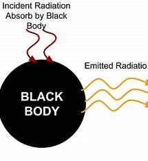
Radiation from Black Bodies
All radiation wavelengths are perfectly absorbed and emitted by the black body. Radiation is released by a black body. According to its temperature. This idea is essential to comprehending how stars and planets emit heat.
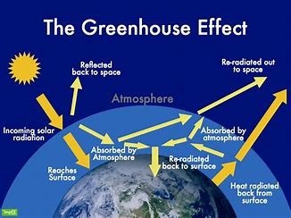
The Greenhouse Effect
The greenhouse effect is a natural atmospheric process that makes Earth habitable by maintaining global temperatures about 33°C warmer than it would otherwise be. This complex interplay of solar radiation and atmospheric gases has become a central focus in climate science due to its intensification from human activities.
The Science Behind the Greenhouse Effect
1. The Radiative Energy Balance
Earth’s climate system operates on a delicate energy equilibrium:
- Incoming Solar Radiation: 340 W/m² average at top of atmosphere
- 31% reflected (albedo)
- 69% absorbed (23% atmosphere, 46% surface)
- Outgoing Thermal Radiation: Longwave infrared emission
- Incoming Solar Radiation: 340 W/m² average at top of atmosphere
2. Natural Greenhouse Effect
- Maintains Earth’s average temperature at ~15°C
- Vital for liquid water existence
- Historical stability (±1°C over 10,000 years)
3. Anthropogenic Enhancement
Industrial Revolution Impact:
- CO₂ levels unprecedented in 800,000 years (ice core data)
- 50% increase in radiative forcing since 1750
Current Energy Imbalance:
- +1.6 W/m² (NASA CERES)
Climate Feedbacks and Amplifiers
1. Water Vapor Feedback
- Warmer air → More H₂O evaporation → Stronger greenhouse effect
- Doubles initial CO₂ warming (most powerful feedback)
2. Albedo Feedbacks
- Ice-Albedo Effect: 0.3 W/m²/decade Arctic amplification
- Cloud Changes: Complex net effect (+/- radiation)
3. Carbon Cycle Perturbations
- Permafrost Thaw: 1,500 billion tons carbon at risk
- Ocean Acidification: 30% pH decrease since 1800s
Global Impact Assessment
1. Temperature Records
- +1.2°C since 1880 (NASA GISS)
- 2023: Hottest year in 125,000 years (proxy data)
2. Extreme Weather Intensification
- Heatwaves: 5x more likely (IPCC AR6)
- Precipitation: +7% intensity per °C (Clausius-Clapeyron)
3. Cryospheric Changes
- Arctic Sea Ice: -13% per decade (NSIDC)
- Glaciers: Lost 267±16 Gt/year (2000-2019)
Technological and Policy Solutions
1. Mitigation Strategies
- Carbon Capture: DAC plants removing 4,000 tons/year
- Renewable Energy: Solar PV efficiency now >22%
- Methane Reduction: Potential to avoid 0.3°C by 2040s
2. Adaptation Measures
- Coastal Defenses: $400 billion needed annually
- Climate-Resilient Crops: Drought-tolerant varieties
3. Global Agreements
- Paris Accord: 196 signatories targeting <2°C
- Kigali Amendment: Phasing down HFCs
Future Climate Projections
1. IPCC Scenarios
Scenario | 2100 Warming | Sea Level Rise |
SSP1-1.9 | +1.4°C | 0.3-0.6 m |
SSP2-4.5 | +2.7°C | 0.4-0.8 m |
SSP5-8.5 | +4.4°C | 0.6-1.3 m |
2. Tipping Points at Risk
- AMOC Collapse: 34% weakening since 1850
- Amazon Dieback: 17% already deforested
- Permafrost Carbon Release: Possible at +2°C
The greenhouse effect represents both:
- A lifesaving natural phenomenon
- An accelerating climate challenge
Addressing its anthropogenic enhancement requires:
- Advanced climate modeling
- International cooperation
- Clean energy transitions
- Ecosystem preservation
Optics and Sounds
Optics and acoustics represent two fundamental branches of wave physics that govern how we perceive our environment. While optics deals with electromagnetic radiation (primarily visible light), acoustics focuses on mechanical pressure waves (sound). Together, these phenomena explain everything from rainbow formation to concert hall acoustics.
Fundamental Principles of Light
Wave-Particle Duality
- Electromagnetic Spectrum: 400-700nm visible range
- Photon Energy: E = hc/λ (h=6.63×10⁻³⁴ J·s)
- Speed of Light: 299,792,458 m/s (vacuum)
Geometric Optics
Lens Formulas
1f=1do+1dif1=do1+di1
- f = focal length
- dₒ = object distance
- dᵢ = image distance
Optical Instruments
- Microscopes: 2000x magnification
- Telescopes: 10m primary mirrors (Keck)
- Cameras: f/1.2 to f/22 aperture range
1.3 Modern Optical Technologies
Fiber Optics
- Total internal reflection (critical angle θ_c)
- Low-loss silica fibers (0.2 dB/km)
- 100+ Tbps data transmission
Holography
- Laser interference patterns
- Security applications (credit cards)
Photonic Crystals
- Bandgap engineering
- Optical computing applications
Acoustics – The Science of Sound
2.1 Fundamentals of Sound Waves
Wave Characteristics
v=fλv=fλ
- v = speed (343 m/s in air)
- f = frequency (20Hz-20kHz audible)
- λ = wavelength
Sound Intensity
β=10log10(II0)β=10log10(I0I)
- I₀ = 10⁻¹² W/m² (threshold)
2.2 Psychoacoustics
Human Hearing
- Frequency Range: 20Hz-20kHz
- Dynamic Range: 120dB (pain threshold)
- Masking Effects: Critical bands
Sound Perception
- Loudness: Phon scale
- Pitch: Mel scale
- Localization: 5° accuracy (binaural)
2.3 Architectural Acoustics
Reverberation Time
RT60=0.161VART60=A0.161V
- V = room volume
- A = total absorption
Concert Hall Design
- Early Reflections: <50ms delay
- Diffusion: Schroeder diffusers
- Noise Criteria: NC-25 for studios
Optical Breakthroughs
- Metamaterials: Negative refraction
- Quantum Optics: Entangled photons
- Adaptive Optics: Corrects atmospheric distortion
Acoustic Innovations
- Sonic Levitation: 40kHz standing waves
- Acoustic Cloaking: Gradient index materials
- Infrasound Monitoring: Volcano prediction
From enabling global communications to diagnosing medical conditions, understanding optical and acoustic phenomena drives technological progress across:
- Information Technology
- Medical Diagnostics
- Environmental Monitoring
- Entertainment Systems

ELECTRICITY AND MAGNETISM
1. Electric Charge: The Foundation of Electricity
1.1 Nature of Electric Charge
Basic Properties:
- Quantized in units of electron charge (1.6×10⁻¹⁹ C)
- Conservation law (net charge remains constant)
- Two types: Positive (protons) and Negative (electrons)
Triboelectric Series:
Material | Charge Affinity |
Glass | + |
Human Hair | + |
Paper | Neutral |
Rubber | – |
Teflon | – – |
1.2 Charge Interactions
Coulomb’s Law:
F=keq1q2r2F=ker2q1q2
- kₑ = 8.99×10⁹ N·m²/C²
- Force: Attractive for opposite, repulsive for like charges
1.3 Practical Applications
- Capacitors: Store energy (up to 10,000 F in supercapacitors)
- Electrostatic Precipitators: Remove 99% of particulates
- Photocopiers: Use charged toner particles
2. Electric Current: The Flow of Charge
2.1 Current Fundamentals
Definition:
I=dQdtI=dtdQ
- 1 Ampere = 1 Coulomb/second
- Drift velocity: ~0.1 mm/s in copper wires
2.2 Current Types Comparison
Parameter | DC | AC |
Direction | Constant | Sinusoidal (50/60Hz) |
Generation | Batteries | Generators |
Transmission Loss | Higher | Lower |
Applications | Electronics | Power Grids |
2.3 Current Applications
DC Systems:
- Electronics (0-48V)
- Electric vehicles (400V+)
AC Systems:
- Household (120/240V)
- Industrial (480V 3-phase)
3. Voltage: The Electrical “Pressure”
3.1 Potential Difference
Definition:
V=WqV=qW
- 1 Volt = 1 Joule/Coulomb
- Analogous to water pressure
3.2 Voltage Ranges
Category | Range | Example |
Extra Low | <50V AC | USB ports |
Low | 50-1000V AC | Household |
High | >1000V | Power lines |
3.3 Transmission Efficiency
Power Loss:
- Ploss=I2RPloss=I2R
High Voltage Advantage:
- 765kV lines lose only 2%/1000km
4. Resistance: Opposing Current Flow
4.1 Resistance Factors
R=ρLAR=ρAL
Resistivity (ρ):
Material | ρ (Ω·m) |
Silver | 1.59×10⁻⁸ |
Copper | 1.68×10⁻⁸ |
Silicon | 6.4×10² |
Glass | 10¹⁰-10¹⁴ |
4.2 Temperature Effects
- Metals: Resistance increases (~0.4%/°C for Cu)
- Semiconductors: Resistance decreases
4.3 Practical Components
- Resistors: 1Ω-10MΩ (5% to 0.1% tolerance)
- RTDs: Platinum (100Ω at 0°C)
- Thermistors: β=3000-5000K
5. Ohm’s Law: The Fundamental Relationship
5.1 Mathematical Formulation
V=IRV=IR
Power Corollary:
- P=IV=I2R=V2RP=IV=I2R=RV2
5.2 Circuit Analysis Examples
1. LED Circuit:
- Vₛ = 9V, Vₗₑₜ = 2V, I=20mA
- R = (9-2)/0.02 = 350Ω
2. Power Calculation:
- 120V, 60W bulb → R = 120²/60 = 240Ω
6. Circuit Configurations: Series vs Parallel
6.1 Series Circuits
Characteristics:
- Single current path
- Voltage divides
- Rₜ = R₁ + R₂ + … + Rₙ
Applications:
- Christmas lights (if one fails, all fail)
- Battery cells (1.5V × n)
6.2 Parallel Circuits
Characteristics:
- Multiple current paths
- Current divides
- 1/Rₜ = 1/R₁ + 1/R₂ + … + 1/Rₙ
Applications:
- Household wiring
- Computer power supplies
6.3 Comparison Table
Property | Series | Parallel |
Current | Same | Divides |
Voltage | Divides | Same |
Resistance | Increases | Decreases |
Failure Mode | Cascade | Isolated |
7. Advanced Concepts
7.1 Kirchhoff’s Laws
- Current Law: ΣIₙ = 0 at nodes
- Voltage Law: ΣVₙ = 0 in loops
7.2 Superposition Theorem
- Analyze multiple sources separately
- Combine results linearly
7.3 Thévenin Equivalents
Simplify complex networks to:
- Vₜₕ (open-circuit voltage)
- Rₜₕ (equivalent resistance)
8. Practical Applications
8.1 Residential Wiring
Standard Circuits:
- 15A @ 120V (1.8kW)
- 20A @ 240V (4.8kW)
8.2 Electronic Design
Voltage Dividers:
- Vout=VinR2R1+R2Vout=VinR1+R2R2
Current Limiting:
- For LEDs and IC protection
8.3 Power Systems
Three-Phase Power:
- 415V line-to-line (240V phase-neutral)
- 50kW+ industrial loads
9. Safety Considerations
9.1 Shock Hazards
Current (AC) | Effect |
1mA | Perception |
10mA | Muscle lock |
100mA | Fatal |
9.2 Protection Devices
- Circuit Breakers: Magnetic/thermal (B, C, D curves)
- GFCIs: Trip at 5mA imbalance
- Surge Protectors: Clamp at 330V
Understanding these fundamental concepts enables:
- Efficient circuit design
- Troubleshooting electrical systems
- Innovative electronic developments
- Safe power utilization

THERAPEUTIC ACTION OF DRUGS
Gastrointestinal Medications
1.1 Acid Control Therapies
Proton Pump Inhibitors (PPIs)
Drug | Bioavailability | Half-life | Peak Effect | Key Features |
Esomeprazole | 50-90% | 1.3 hr | 2-4 hr | (S)-isomer of omeprazole |
Pantoprazole | 77% | 1.9 hr | 2.5 hr | CYP450-independent metabolism |
Rabeprazole | 52% | 1.5 hr | 3.6 hr | Fastest onset among PPIs |
Clinical Considerations:
- Duration: 14-day treatment courses common
- Adverse Effects: 0.1-1% risk of C. difficile infection
- Market Size: $13.9 billion globally (2023)
H2 Receptor Antagonists
- Ranitidine: Withdrawn (2020) due to NDMA contamination
- Cimetidine: Potent CYP450 inhibitor (avoid with warfarin)
1.2 Comparative Efficacy
Parameter | PPIs | H2 Blockers |
pH >4 Duration | 14-21 hr | 8-10 hr |
Nocturnal Acid Breakthrough | 70% control | 30% control |
Healing Rate (GERD) | 85-95% | 50-70% |
Section 2: Antihistamines and Allergy Management
2.1 Evolution of Antihistamines
Generation | Example | Sedation Risk | QT Risk |
1st | Brompheniramine | High | Low |
2nd | Terfenadine | Low | High (withdrawn) |
3rd | Fexofenadine | Minimal | None |
Pharmacokinetics:
- Fexofenadine: Tmax=2.6 hr, high P-gp substrate
- Bilastine: Newest (2010), food-independent absorption
2.2 Clinical Applications
- Chronic Urticaria: 180mg fexofenadine daily
- Allergic Rhinitis: Intranasal antihistamines (azelastine)
Section 3: Neuroactive Agents
3.1 Anxiolytics
Drug | Onset | Duration | Key Risk |
Alprazolam | 30 min | 6-12 hr | High abuse potential |
Clonazepam | 1 hr | 18-50 hr | Withdrawal seizures |
Prescribing Trends:
- 13% decrease in benzodiazepine scripts (2015-2020)
- 62 million alprazolam prescriptions (2022, US)
3.2 Opioid Analgesics
Drug | Potency (vs morphine) | DEA Schedule |
Oxycodone | 1.5x | II |
Fentanyl | 100x | II |
Carfentanil | 10,000x | Not approved |
Epidemiology:
- 80,411 opioid deaths (2021, CDC)
- Naloxone distribution: 1.2 million kits (2022)
Section 4: Antimicrobial Agents
4.1 Antibiotic Classes
Class | Example | Spectrum | Resistance Concern |
Carbapenems | Meropenem | Gram±, anaerobes | NDM-1 metallo-β-lactamase |
Glycopeptides | Telavancin | Gram+ | VanA/B/C genes |
Polymyxins | Colistin | Gram- | mcr-1 plasmid |
Clinical Pearls:
- Azithromycin: 5-day Z-pack remains popular
- Doxycycline: First-line for tick-borne illnesses
4.2 Antifungal/Antiviral
- Amphotericin B: Gold standard but nephrotoxic
- Remdesivir: COVID-19 treatment shortening recovery
Section 5: Reproductive Health
5.1 Contraceptive Options
Type | Formulation | Pearl |
COCP | Ethinylestradiol + levonorgestrel | 99.7% effective |
POP | Norethindrone | Lactation-safe |
Emergency | Ulipristal acetate | 5-day window |
5.2 Medical Abortion
- Mifepristone: Progesterone receptor antagonist
- Misoprostol: 800μg buccal dose
- Efficacy: 95-98% success <9 weeks gestation
Section 6: Emerging Therapies
6.1 Novel Mechanisms
- Vonoprazan: Potassium-competitive acid blocker (Japan)
- Oliceridine: Biased μ-opioid agonist (2020 FDA approval)
6.2 Biosimilars
- Adalimumab biosimilars: 5 approved in 2023
- Cost Savings: 25-30% vs originators
Comparative Tables
PPI Metabolism Pathways
Drug | CYP2C19 Dependent | CYP3A4 Pathway |
Omeprazole | 85% | 15% |
Lansoprazole | 75% | 25% |
Dexlansoprazole | 50% | 50% |
Opioid Receptor Binding
Drug | μ-Affinity (nM) | δ-Affinity |
Morphine | 1.8 | Weak |
Fentanyl | 0.39 | None |
Buprenorphine | 0.21 | Partial agonist |
Safety Considerations
Black Box Warnings
- PPIs: Long-term fracture risk
- Benzodiazepines: Respiratory depression
- Colistin: Neuro/nephrotoxicity (>5mg/kg/day)
Drug Interactions
- Fluconazole + Fexofenadine: 164% AUC increase
- Clarithromycin + Midazolam: Contraindicated
Modern pharmacology offers:
- Precision-targeted therapies (e.g., esomeprazole)
- Safer alternatives (3rd-gen antihistamines)
- Life-saving interventions (colistin for XDR infections)
CHEMICALS IN FOOD
Natural Sweetener Options
Stevia (Rebaudioside A)
- Extraction: From Stevia rebaudiana leaves
- Properties: 200-400x sweeter than sugar
- Regulatory Status: GRAS in US since 2008
- Market Growth: $790 million (2023), 8.1% CAGR
Monk Fruit Extract
- Source: Siraitia grosvenorii
- Advantage: Zero glycemic impact
- Limitation: 80% blended with erythritol
Physiological Impacts
- Blood Sugar: No acute glycemic spike (FDA-approved for diabetics)
- Gut Microbiome: Sucralose may reduce beneficial bacteria by 50%
- Weight Management: Mixed evidence on long-term efficacy
Natural Preservation Alternatives
- Rosemary Extract: Rich in carnosic acid
- Nisin: Bacteriocin from Lactococcus lactis
- Vinegar: 4% acetic acid effective against E. coli
Regulatory Landscape
- EU: 43 approved preservatives (Regulation EC 1333/2008)
- US: 32 CFR-approved chemical preservatives
- Japan: Allows 50+ including unique isothiocyanates
Section 3: Controversial Food Additives
Titanium Dioxide (E171)
Applications:
- White pigment in candies (Skittles®)
- Toothpaste opacifier
Safety Concerns:
- 2021 EFSA reclassification as “not safe”
- Nanoparticle (<100nm) accumulation in gut
- Market Impact: Banned in EU (2022), alternatives like calcium carbonate emerging
Bisphenol A (BPA)
- Usage: Polycarbonate plastics, epoxy resins
- Exposure:
- 2-10 μg/kg/day from canned foods
- 90% population has detectable levels
Regulatory Actions:
- Banned in baby bottles (US 2012, EU 2011)
- 10μg/kg/day TDI set by EFSA (2023)
Emerging Concerns
- Phthalates: Plasticizers migrating from packaging
- PFAS: “Forever chemicals” in grease-proof papers
- Carrageenan: Debate on intestinal inflammation
Flavor Enhancers
4.1 Common Flavor Additives
Additive | Source | Umami Strength | Daily Limit |
MSG | Fermented starch | 100x glutamate | No ADI set |
Disodium Inosinate | Meat extracts | 50x nucleotides | 0.5g/kg |
Yeast Extract | S. cerevisiae | Natural alternative | Unlimited |
4.2 “Clean Label” Movement
- Demand: 64% consumers prefer natural flavors
- Innovations: Fermented flavors from fungi
- Challenges: Cost 2-5x synthetic equivalents
Section 5: Safety Evaluation
5.1 Toxicological Testing
- Acute Toxicity: LD50 determinations
- Chronic Studies: 2-year rodent bioassays
- NOAEL: No Observed Adverse Effect Level
5.2 Risk Assessment Framework
- Hazard Identification
- Dose-Response Analysis
- Exposure Assessment
- Risk Characterization
5.3 Major Studies
- Ramazzini Institute: Aspartame carcinogenicity claims
- French NutriNet-Santé: Ultra-processed food risks
- FDA CFSAN: Ongoing post-market surveillance
Section 6: Consumer Guidance
6.1 Reading Labels
- E-numbers: EU coding system (E200-E299 preservatives)
- Organic Standards: Prohibit most synthetic additives
6.2 Reduction Strategies
- Whole Foods: <5% contain additives vs 60% processed foods
- Home Preservation: Pickling, fermenting, freezing
6.3 High-Risk Groups
- Children: Lower body weight = higher exposure/kg
- Pregnant Women: BPA crosses placental barrier
- Allergy Sufferers: Sulfites trigger asthma
Comparative Tables
Sweetener Metabolic Fate
Type | GI Tract Absorption | Metabolism | Excretion |
Aspartame | 100% | Hepatic (esterases) | Renal |
Sucralose | 15% | None | 85% fecal |
Steviol | 100% | Colonic (bacteria) | Renal |
Preservative Efficacy
Agent | Bacteria | Yeasts | Molds |
Sorbate | ++ | +++ | +++ |
Benzoate | +++ | ++ | + |
Natamycin | – | +++ | ++++ |
Modern food additives present:
- Technological benefits (shelf-life extension, flavor enhancement)
- Health trade-offs (potential long-term risks)
- Regulatory challenges (global harmonization needed)
Informed choices require understanding:
- Additive functions
- Exposure levels
- Individual risk factors

CLEANSING AGENTS
The Science of Cleaning Agents
1.1 Traditional Soaps vs Modern Detergents
Soap Chemistry Fundamentals
Saponification Reaction:
Triglyceride+NaOH→Glycerol+SoapTriglyceride+NaOH→Glycerol+Soap
Common Soap Salts:
Soap Molecule | Source | Hard Water Performance |
Sodium palmitate | Palm oil | Poor (scum forms) |
Sodium stearate | Tallow | Moderate |
Sodium oleate | Olive oil | Better |
Palm Oil Controversy:
- 66% global soap production uses palm derivatives
- 8% annual deforestation rate in Indonesia/Malaysia
- RSPO-certified sustainable palm oil now available
Synthetic Detergents Evolution
Generation | Example | Key Advancement |
1st (ABS) | Branched alkylbenzene sulfonate | Poor biodegradability |
2nd (LAS) | Linear alkylbenzene sulfonate | 90% biodegradable |
3rd (AE) | Alcohol ethoxylates | Highly biodegradable |
Modern Formulations:
- Enzymatic detergents: Protease/lipase blends (37°C optimal)
- Biosurfactants: Rhamnolipids from Pseudomonas (0.1% concentration effective)
1.2 Environmental Impact Analysis
Phosphate Regulations Timeline
Year | Region | Limit | Impact |
1972 | US (Great Lakes) | <0.5% P | 75% reduction in algal blooms |
2013 | EU | 0.3g P/wash | Zeolite alternatives adopted |
2017 | China | 1.1% P | Gradual phase-out |
Microplastic Bans:
- EU: Complete ban (2025) on <5mm plastics
- US: Microbead-Free Waters Act (2015)
- Alternatives: Apricot shells, jojoba wax beads
Section 2: Essential Household Chemicals
2.1 Food & Beverage Components
Nutritional Chemistry
Compound | Daily Value | Function | Overconsumption Risk |
NaCl | <5g (WHO) | Nerve conduction | Hypertension |
Sucrose | <25g (added) | Energy source | Obesity, diabetes |
Caffeine | 400mg max | Adenosine blockade | Insomnia |
MSG Science:
- Umami receptor activation (T1R1/T1R3)
- 0.1-0.8% optimal in foods
- No conclusive evidence for “Chinese Restaurant Syndrome”
2.2 Medicinal Compounds
Pain Relievers Comparison
Drug | Onset | Duration | COX Inhibition | Risk |
Paracetamol | 30min | 4-6hr | Central only | Liver toxicity |
Aspirin | 45min | 4-6hr | COX-1>COX-2 | Bleeding |
Ibuprofen | 20min | 6-8hr | COX-1≈COX-2 | GI upset |
Antibiotic Development:
- Penicillin G: 1-4 million units typical dose
- Resistance Crisis: 1.27 million deaths (2019) from resistant infections
2.3 Household Chemistry
Disinfectant Efficacy
Agent | Concentration | Kill Time (E. coli) | pH Sensitivity |
NaClO (6%) | 0.5% | 1min | >10 loses efficacy |
H₂O₂ (3%) | Undiluted | 5min | Stable |
Ethanol | 70% | 30sec | Optimal at neutral |
Baking Soda Uses:
- Cleaning: 1:1 paste for scrubbing
- Fire Extinguisher: Decomposes at 50°C releasing CO₂
- Odor Neutralizer: pH 8.4 absorbs acidic volatiles
Section 3: Controversial Chemicals in Spotlight
3.1 Environmental Pollutants
PFAS “Forever Chemicals”
- Structure: 4,700+ variants of fluorinated chains
- Persistence: Half-life >5 years in body
- Regulation:
- EPA MCL: 4ng/L for PFOA/PFOS
- EU REACH: Proposed ban (2023)
Microplastic Invasion:
- Sources: 35% from synthetic textiles
- Human Exposure: 0.1-5g weekly intake
- Removal Tech: Magnetic nano-polymers (90% capture)
3.2 Health Controversies
Glyphosate Debate
- IARC: Class 2A probable carcinogen
- EPA: “No risks when used properly”
- Global Use: 800,000 tons annually
BPA Alternatives:
Replacement | Estrogenic Activity | Thermal Stability |
BPS | 100x less | Similar |
BPF | 10x less | Lower |
Tritan™ | None | Excellent |
Section 4: Emerging Chemical Technologies
4.1 Medical Breakthroughs
mRNA Vaccine Tech
- Lipid Nanoparticles: 70-100nm size range
- Stability: -70°C storage (improving to 2-8°C)
- Efficacy: 95% COVID prevention (initial strains)
CRISPR-Cas9:
- Precision: Single base pair editing
- Therapies: Beta-thalassemia trials (2023)
- Delivery: Viral vectors vs lipid nanoparticles
4.2 Material Science Advances
Graphene Applications
Property | Value | Application |
Strength | 130GPa | Lightweight armor |
Conductivity | 10⁸ S/m | Flexible electronics |
Surface Area | 2630m²/g | Supercapacitors |
Self-Cleaning Surfaces:
- TiO₂ photocatalysis breaks down organics
- Shark-skin inspired micro-patterns (anti-biofouling)
Comparative Analysis Tables
Soap vs Detergent Properties
Property | Soap | Synthetic Detergent |
Biodegradability | 100% | 40-90% |
Hard Water Performance | Poor | Excellent |
Cost | $2-5/kg | $1-3/kg |
pH | 9-10 | 7-9 |
Disinfectant Spectrum
Agent | Bacteria | Viruses | Spores | Toxicity |
Bleach | +++ | +++ | ++ | High |
Alcohol | ++ | ++ | – | Moderate |
H₂O₂ | +++ | +++ | + | Low |
Safety & Regulatory Landscape
Global Chemical Regulations
Region | Framework | Key Requirement |
EU | REACH | 1+ ton/yr requires dossier |
US | TSCA | EPA risk evaluation |
China | MEE | New chemical registration |
Household Chemical Safety
Mixing Risks:
- Bleach + Ammonia → Chloramine gas
- H₂O₂ + Vinegar → Peracetic acid
Storage:
- Original containers, away from children
This comprehensive examination reveals:
- Cleaning product evolution toward sustainability
- Essential chemicals’ dual roles as helpers/hazards
- Emerging technologies solving old problems
Understanding molecular interactions empowers:
- Safer product choices
- Environmental stewardship
- Informed policy decisions